Arctic pollution studied with models and satellite observations in support of the ARCTAS campaign

Increasing anthropogenic pollution and wildfires are the main producers of CO (carbon monoxide) pollution in the Northern Hemisphere. During the NASA ARCTAS field campaign , the ACRESP group used models and satellite data to study the polluted air masses that are transported into the Arctic troposphere, influencing the ecosystem in high northern latitudes and the global radiation and climate. The global chemical transport model MOZART-4 was used to quantify the contribution of CO from different source regions by tagging.

Besides large contributions of anthropogenic pollution, wildfires in the Northern Hemisphere play an important role, especially between April and June, as shown in the animation. This is particularly true of the pollution produced by large Siberian fires in springtime that is transported towards North America, and together with other fires in the Northern Hemisphere, these contribute to the pollution over the entire polar cap.

Figure 1:(Click image to view the animation.) CO pollution from fire emissions between April and June in the Northern Hemisphere using the MOZART-4 model. This excludes South Asian fires that have their main influence in April in mid-latitudes.

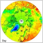
MOPITT (Measurements of Pollution in the Troposphere) satellite retrievals of tropospheric carbon monoxide (CO) over the Arctic from 2000 to 2009 were recently analyzed using the new MOPITT Version 4 Product. While retrievals based on nadir-view thermal-infrared radiances are more challenging in the Arctic compared to the Tropics and midlatitude regions, useful retrievals of CO total column can be obtained in most seasons for most regions within the Arctic. As indicated in the plots below for January, April, July, and October, long-term monthly-mean maps based on MOPITT observations from 2000-2009 demonstrate that (1) total column values usually peak in March/April while dropping to minimum values in August/September and (2) in springtime, the largest monthly-mean total column values appear over the N Pacific Ocean and over N Europe/Russia. Maps of interannual variability (total column standard deviations) demonstrate that (1) variability patterns reveal biomass burning regions, (2) variability is strongest in the NH summer (July), esp. over boreal forests in Siberia and N America, and (3) low values of DFS (Degrees of Freedom for Signal) can suppress possible evidence of geophysical variability (e.g., in January).

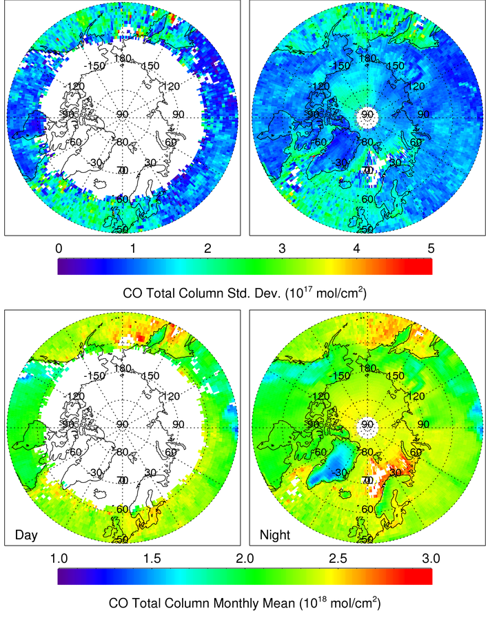January	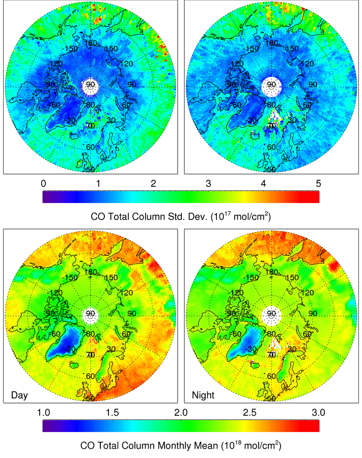April
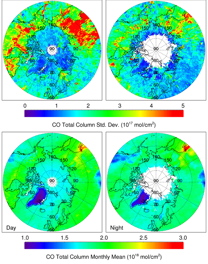July	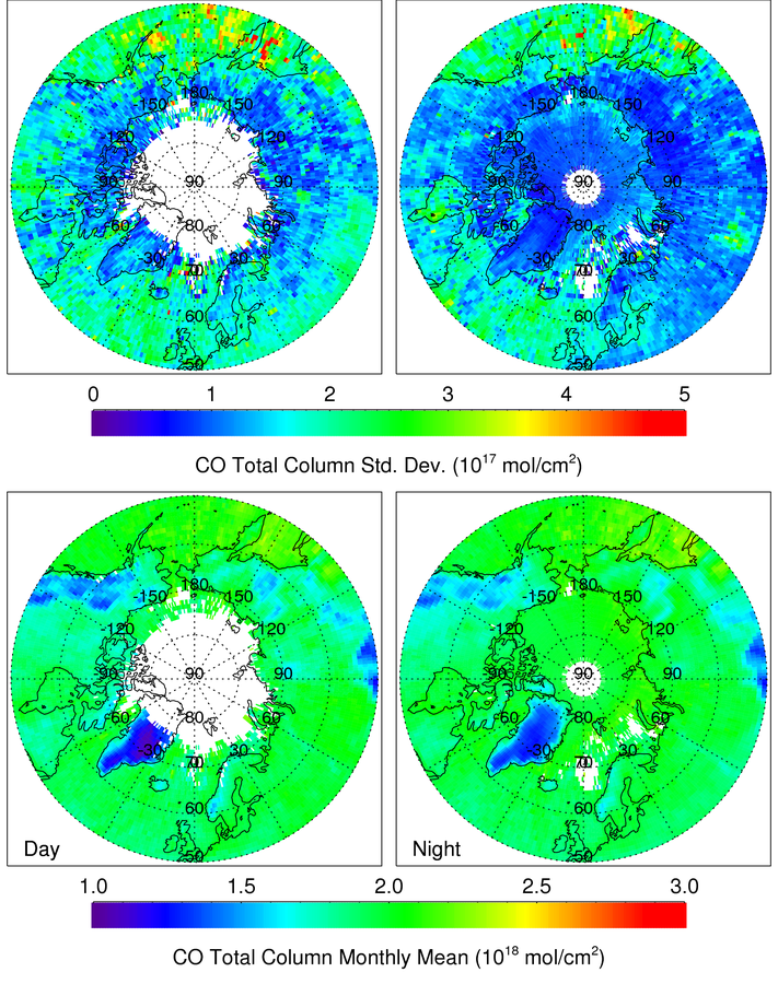October

Figure 2. MOPITT retrievals of tropospheric carbon monoxide by month, 2000-2009. Click to view larger images.